No Free Lunch: Understanding Volatility, Average Prices, and Valuation

As equity compensation valuation experts, we’re always on the lookout for new ideas. We’re also interested in the best ways to implement guidance from the SEC and FASB. Sometimes their guidance allows for significant discretion in our valuation methodologies, in which case we have a professional responsibility to help our clients apply this discretion without creating risk in their financial statements or system of controls.

That’s why we regard novel or atypical approaches with a healthy dose of professional skepticism. The merits, which need to be fundamentally sound, need to outweigh the cost or risk.

Lately there’s been renewed debate about the calculation of volatility, which is an area of substantial discretion—and nuanced complexity—that affects almost all equity compensation instruments. Typically, closing prices are used in the volatility calculation. One idea that has resurfaced is that average stock prices over a period can be used instead. The justification is essentially that since we have to use a daily price, it may make more sense to use the average of all the trades rather than a single, seemingly arbitrary price.

This approach would systematically yield lower fair values that would boost companies’ income statements or allow for more awards to be granted. But it does so in a way that violates core finance and statistical principles and therefore, in our opinion, is not compliant with ASC 718.

To understand why, let’s take a closer look at the two competing models: a traditional volatility calculation based on daily closing prices, and the novel calculation that uses average prices in the calculation.

Comparing Volatility Models

Volatility is a measure of how much a stock price may be expected to move up and down over a period of time. Valuations for GAAP are based on the idea that today’s price is the best guess at the average future price; however, how much the price may move up or down from that average comes from the volatility. For example, we can easily imagine blue-chip companies that are more stable and riskier stocks that fluctuate more.

It’s worth recalling the market mantra of “higher risk, higher reward” and its application here. Volatility is how models measure the risk portion of that statement. Any framework that measures risk without a commensurate attempt to adjust or redefine the reward (or expected return) should be viewed skeptically. If a model is calibrated to a given relationship between risk and reward, changing one and not the other risks disastrous consequences.

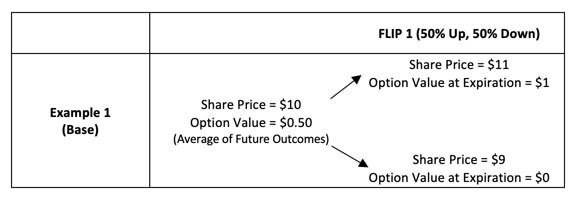
To understand the impact of volatility on valuations, consider a hypothetical company named Coin Flip Enterprises (HTHT). Tonight, the CEO of HTHT will flip a coin. If it comes up heads, the stock price will go to $11. If tails, the stock price will fall to $9. The stock today trades at $10.

We speculate that tomorrow may be a good day for heads, and thus want to buy a one-day option with a strike price of $10. This option should cost $0.50 in our simple world because there’s a 50% chance the stock price goes up and we make $1, and a 50% chance we lose our initial investment and the option expires with no value.

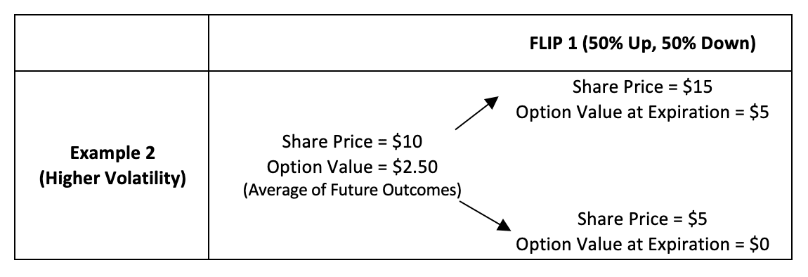
Now imagine that the CEO decides to make a bigger bet, such that the price move will be up or down $5. This is higher volatility or a riskier company, and simple math shows how the volatility increases the option value.

Now it’s obvious that this example is simplified, as indeed a stock moves throughout the day. We can measure how much the stock bounces a few different ways:

• The standard method is to use the value at the end of the day
• An averaging approach looks at prices throughout the day—for example, an average of the high and low, a time weighted average, or a volume weighted average

With these two frameworks in mind, we can analyze whether an average approach can ever yield a superior estimate of volatility. Our results show that GAAP rules, practicality, and the data favor the traditional approach.

**********

How Does the Average-Price Approach Fail in Forecasting? Look at the Gas Pump

Suppose you’re trying to forecast the average price of gasoline next month. And imagine that gas prices have been increasing such that last month’s average price is $3.50 a gallon but today’s price is $4.00 a gallon. We would view the $3.50 average as a fair indication of how the last month has gone, but not as a good predictor of how next month will go.

If we were to predict next month’s average gas price, it would be quite clear that $4.00 is the meaningful number. We wouldn’t assume the price will automatically fall back to $3.50 just because it was the prior month’s average.

Alternatively, if gas prices have been falling and today’s price is $3, we wouldn’t expect an instantaneous rebound.

An average-price volatility calculation implicitly assumes this snap-back effect by measuring movements from an average. This ignores information that’s critical to setting future expectations. It’s why an average-price volatility approach doesn’t work with the valuation models used under ASC 718.

**********

US GAAP Guidance Violated by Average-Price Volatilities

As a first test, let’s look to the authoritative guidance. In SAB Topic 14.D.1, it’s stated that

FASB ASC subparagraph 718-10-55-37(d) indicates an entity should use appropriate and regular intervals for price observations based on facts and circumstances that provide the basis for a reasonable fair value estimate…Company B should select a consistent point in time within each interval when selecting data points.[1]

At best, it’s questionable whether an average price could suit this requirement.

• The average does (potentially) reflect a daily price observation
• The timing of the average is uncertain and inconsistent, so the average price may be closer to market close Monday, market open Tuesday, and midday Wednesday
• While the average price reflects trading activity, it’s quite possible that the stock jumped over an average price and never actually traded at or near the average, especially on a day when news came in midday

Following up on the text of ASC 718 (then known as FAS 123R), consider an SEC staff speech by Alison Spivey in 2005. Spivey points out the key measurement principle and two potentially violating approaches:

When evaluating the alternative methods, we would encourage companies to keep in mind the objective as stated in Statement 123R [ASC 718] to ascertain the assumption about expected volatility that marketplace participants would likely use in determining an exchange price for an option. The staff expects companies to make good faith efforts to determine an appropriate estimate of expected volatility as one of the key assumptions used in determining a reasonable fair value estimate.

We have become aware of two methods for computing historical volatility that we believe will not meet this expectation. The first method is one that weighs the most recent periods of historical volatility much more heavily than earlier periods. The second method relies solely on using the average value of the daily high and low share prices to compute volatility. While we understand that we may not be aware of all of the methods that currently exist today and that others may be developed in the future, we would like to remind companies to keep in mind the objective in Statement 123R [now ASC 718] when choosing the appropriate method.

Having experienced the industry practices at that time, we were aware that such an averaging approach was used, or attempted, by some valuation providers. The result was a consistently lower volatility. However, auditors were unwilling to accept it even before Spivey’s speech effectively ended the practice.

More recently, we’ve seen discussion of a volume weighted average price, or VWAP, which takes an average of all trades during the day based on the number of shares in each trade.[2] On its face, we believe it’s quite apparent that a VWAP fails to meet the SEC’s expectations in exactly the same way as a high-low average price. However, in the interest of completeness, we can consider any method through the three lenses key to SEC and GAAP compliance: market usage, mathematical acceptability, and consistency with the underlying data.

Market Usage of Average-Price Volatilities Appears Lacking

Moving from the guidance, we look to the marketplace. While we haven’t performed a comprehensive market survey, our team at Equity Methods includes people who have worked on options and similar instruments for two of the Big Four, within hedge funds, on the option trading floor, as an expert witness in significant litigation, and through multiple academic finance, quantitative, and financial engineering programs. None of us have seen the use of an averaging method to calculate a volatility rate to be applied to longer term options by traders or other market users. An examination of academic literature reveals only two examples of a calculation wherein a return was calculated based on average prices for the calculation of volatility—though neither supports such a method’s use in practice.[3]

Additionally, we note that a substantial amount of trading in derivatives is on indices. Simply stated, because there is not trading in the index like in individual stocks, no VWAP exists. If this were indeed a superior measure, we would expect traders would have spent much time and energy to capture the arbitrage opportunity this would imply. As far as we know, no one has built any model for this, and data services report no estimate for the VWAP of indices.

A counterargument may be that an average price would consider actual trading activity throughout the day better than one potentially arbitrary price. But it’s impossible to trade at an average price, which casts doubt on the argument that it would represent trading activity better. First, the market may never have seen this price in an actual trade. Second, you wouldn’t know the average until the end of the day, potentially hours after it passed on a big move day. So while the average may reflect where investors bought and sold their shares, it’s not even possibly reflective of an individual investor’s position over the period.

Statistical Problems with Average-Price Volatility

If the GAAP guidance and our market knowledge aren’t convincing enough, consider the statistical properties of average-based volatility. If the statistics were superior to the traditional model, then pushing a shift in industry practices may be warranted. However, a statistical analysis led us to find the opposite is true.

The crux of the problem has to do with two simple statistical principles regarding volatility. The first is that volatility is calculated based on squared stock movements. As a result, one big price movement will have a dramatically bigger impact on volatility than two smaller moves, even if the total effect on price over time is the same. The second is how volatility is applied. When we apply a Black-Scholes or lattice model, the models assume the best forecast of tomorrow’s price is the last price today, and there’s no other information that would give us a better forecast at that time.

In this section, we break out three details of the volatility calculation to show that using any sort of average volatility is subject to problems. If you’re interested in the quantitative details, hopefully you’ll find this readable even without a degree in statistics. Otherwise, go ahead and skip to the Testing the Models section.

Inconsistent Timing

The first concern we note is the inconsistent period between price observations, which is related to the problem the SEC pointed out. Consistent observations are what allow us to use a simple formula to annualize the observations into a single annual measure. The formula is the standard deviation of daily returns multiplied by the square root of 252, regardless of how many observations we have. This is because there are an average of 252 trading days in a year. Weekly and monthly returns use the square roots of 52 and 12, respectively, for the same type of reason. This is based on every observation having the same weight in the time series.

Although there are ways to calculate the time series volatility based on differently sized intervals, the process is laborious and needs careful consideration of the different time intervals to make the result continuous. And because the average price doesn’t reflect an observation at a particular time, applying this math to project future “point in time” pricing is impossible.

Return Splitting, Prediction, and Volatility

Proponents of average-price volatilities note that the resulting volatility estimate just so happens to return lower results in almost all cases. This fact, which seems too good to be true, is due to a structural issue with the model. A key reason averaging tends to lower volatility is the fact that stocks can rise or fall throughout the day. Therefore, using an average will split the movement of a single day of large returns (when significant news arises) across two days.

Consider a case where a stock moves from $10 to $11 one day, then stays flat the next. In an average approach, it seems to move $0.50 a day. Further, if the stock moves up on day two, we would know for a fact it will go up another $0.50 on day three.

This is a problem. We said earlier that volatility was a measure of how much a stock could move, but we couldn’t know a direction. If we were to use an average price, we could predict perfectly where the stock is going to move, since we’d have chosen to ignore available information such as current trading prices.

This violates a fundamental assumption in all standard valuation models discussed in ASC 718. These models assume that returns from day to day are random, or that we can’t predict tomorrow’s price or returns based on information available today. This underlying concept is known as the “random walk.” Average price measures ignore the random walk. The result is a volatility measure with an implicit downward bias, meaning that the finding of a lower resulting volatility is a built-in feature of the model due to an error.[4]

__________

Average-price volatilities ignore the random walk, a fundamental assumption in all standard valuation models discussed in ASC 718.

__________

Figures 1 and 2 show an example. Imagine HTHT is trading at exactly $10 for five consecutive days. On the sixth day, midway through the trading day, the stock falls from $10 to $9, and the price immediately stabilizes. All trading through the end of day 10 is now at $9.

Using the day-end model, the stock returns are 0% for each day except for day six, while day six is a drop of 10%. If we use an average, however, day six is a drop of 5% from $10 to $9.50 and day seven is a drop of just over 5% from $9.50 to $9. In other words, by using an average, we’ve split the big price drop over two days. Volatility as a result falls from 53% to 35%. This is a material consistency problem for the models using that volatility.

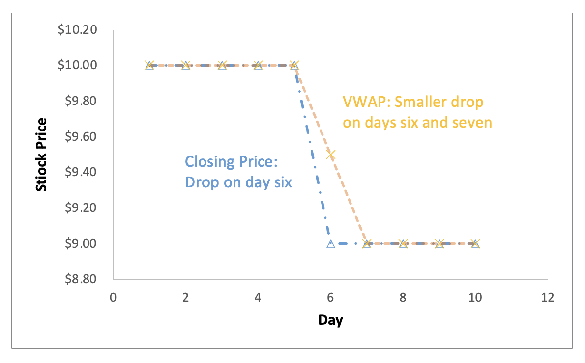
Figure 1: VWAP vs. Closing Stock Price Measurement

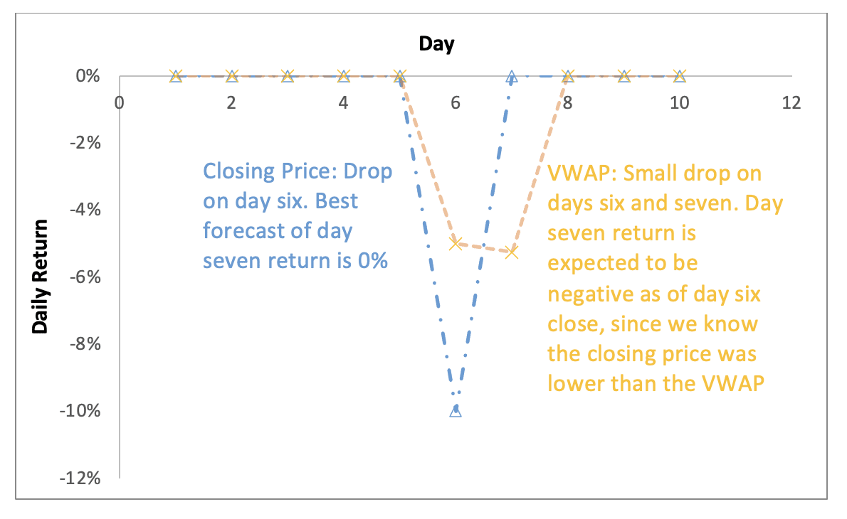
Figure 2: VWAP vs. Closing Stock Price Return Measurement

In reality, we don’t know how a stock is going to move the next day, and the measurement of volatility should reflect that. We do know, however, that the closing price is a much better estimate of tomorrow’s price than an average price is. Imagine some bad news came an hour before market close and the market for a stock immediately dropped from $50 to $40. The average price series will be somewhere in between, since most of the day’s trading was before the news. But if you were to guess where the stock would open tomorrow, you would guess $40. The average is, quite literally, stuck in the past and therefore not a great predictor.[5]

For a real-world example, we looked at Apple’s returns over 2022. In this case, Apple had four days where the stock price moved over 6%, three positive and one negative. The largest changes were +8.5% and +6%. The volatility was 35.5%. If instead we base the returns on the volume-weighted average price calculated over each day, the return tops 6% only once. The volatility falls to 30%, a drop of over 15%!

In fact, in an analysis of the S&P 500, we see that the volatility falls using a VWAP over 99% of the time. This drives home the fact that the approach isn’t simply an alternative. There’s something fundamentally different about it that warrants skepticism.

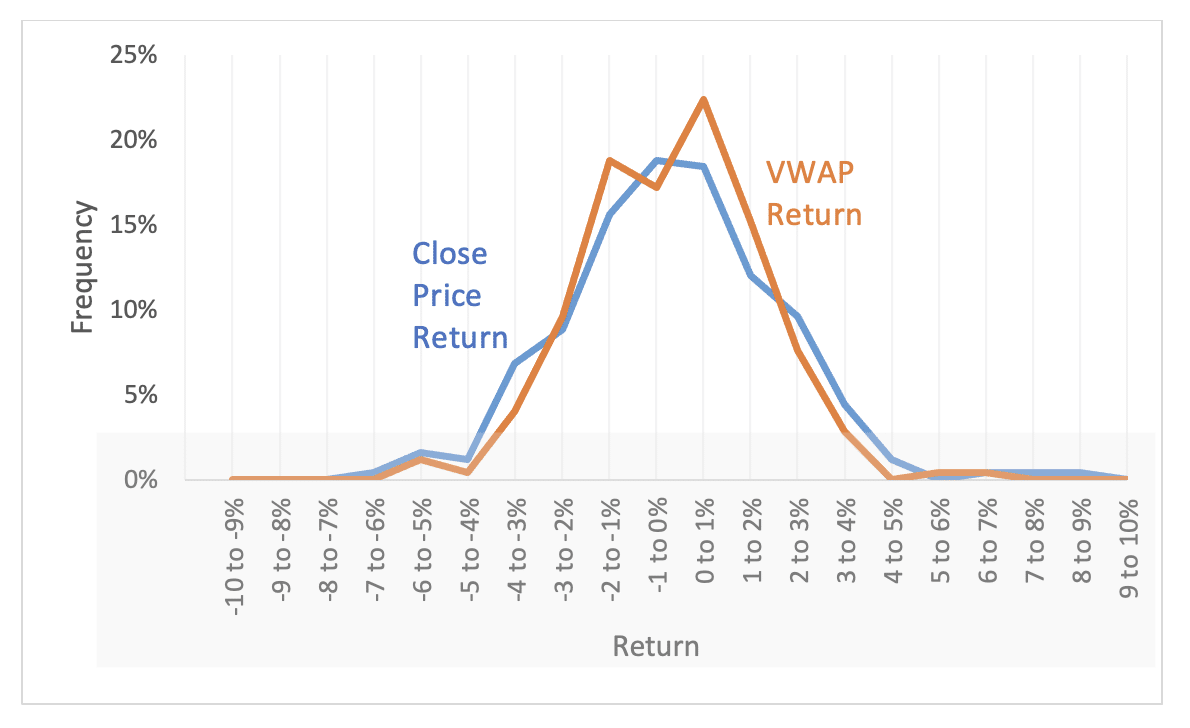
Figure 3: Apple’s Return Frequency under Both Measures

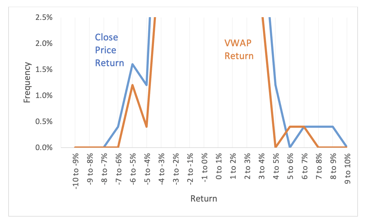
Figure 4: Breakout Showing Differences in Outsized Returns

Autocorrelation and Predictive Power of Returns

Let’s zero in on the random walk assumption and how an average-price volatility breaks the randomness by hiding information about future prices.

We can directly test this using our Apple data. Remember that the model assumes that the best guess of the day-to-day stock movement is random, and that we have no additional knowledge of what might happen. If this is true, an investor cannot profit from a strategy trading based only on past prices. This principle is known as the efficient market hypothesis.

Our testing uses a correlation statistic,[6] which tells us how well today’s return may predict tomorrow’s. This statistic ranges from -1 (two variables move in equal and opposite directions) to 1 (the two are always identical). A value of 0 means tomorrow’s price is completely independent of today’s—it’s random—and that’s how standard models work. In reality, we routinely see that there’s a correlation of end of day returns of around -2%, a very weak relationship. Using an average, however, this figure is around 15%.[7]

Another way to think about it is to consider a hypothetical trader who was able to buy the stock at the VWAP on days the return was positive and sell on days the return was negative, holding until the subsequent day’s average. This hypothetical trader would make a healthy return—almost doubling their money over the course of a year. Of course, we’ve already discussed that this strategy is impossible because you can’t knowingly trade the VWAP while it’s a relevant price. For our typical trader facing market prices, the strategy is worthless, exactly as we would expect.

Testing the Models

Stepping further into analysis of actual market behavior, we can use the fact that volatility is a prediction of a future distribution to analyze the quality of the estimate. We do this by comparing the implied forecast from a volatility measure against actual market returns over a large number of estimates.

Why is this a good test? Volatilities are a measure of how much stocks are expected to move over time and define a distribution. While we may measure this by day, month, or even fraction of a second, our goal is to use this to see what this forecast range looks like over a longer period. If you went to trade with distributions that were too tight, based on volatilities smaller than reality, you would be poised to sell every option you could. In this case, you would face massive losses as everything moved more than you forecasted as reasonable.

__________

If you went to trade with distributions that were too tight, based on volatilities smaller than reality, you would be poised to sell every option you could. In this case, you would face massive losses as everything moved more than you forecasted as reasonable.

__________

We run our test by forecasting a range of potential stock returns that we would expect to occur (say) 95% of the time. Under a normal distribution of returns, you would expect a return within one standard deviation[8] of the forecast 68% of the time and within two standard deviations 95% of the time. So a stock with a price of $100 in an idle market, with volatility of 30%, should be between $74 and $135 68% of the time and $55 and $182 95% of the time.[9]

For our test, we analyzed the returns of the S&P 500 components relative to their forecasted ranges based on both standard and average-price volatility measures. The results show what we suspected. Actual stock returns don’t behave quite like our normal distribution, due to fat tails in the distribution (or kurtosis, for people who prefer SAT words). However, the use of average-price volatilities resulted in much-too-tight forecast ranges. For both the one standard deviation (68%) and two standard deviation (95%) ranges, the likelihood of being outside the best guess interval is more than 10% too high using the VWAP, again showing this range is too tight relative to end-of-day returns.[10]

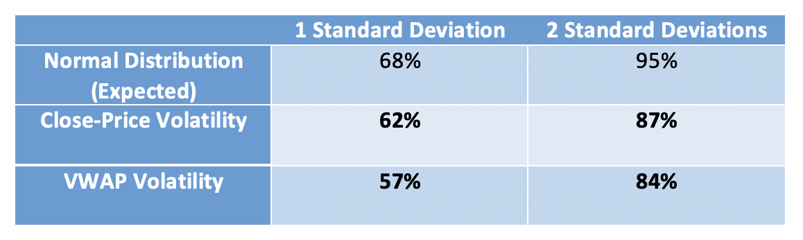
Table 1: Percentage of Data within Return Range Limits

This table shows the frequency of stock returns landing within a given range based on the estimated volatility. VWAP volatility provides a synthetically lowered volatility, resulting in more observations falling outside of the forecast range.

But What If The Target Measure Is a VWAP?

Several of our clients use VWAP rather than closing prices as their variable for vesting and have asked if this makes a difference. The short answer is no, the volatility should still be based on close prices. Indeed, because the closing price is still the best predictor of future prices, it doesn’t matter if we’re forecasting the closing price, opening price, high/low average, or any other metric. The most indicative move will be that of an observation at the same time each day, which avoids these issues.[11]

Conclusion

When it comes to accounting valuations, carefully consider any changes before going all in. This is doubly important when something seems too good to be true, like a near-guaranteed reduction in income statement expense. In general, we believe that any seeming advantages of average-based volatility are based on it being mismatched to the model it’s using, and thus prone to understating option values in a way that’s not compliant with GAAP. A well-reasoned, objective statistical and historical analysis show this to be true for the recently proposed novel methodology of VWAP volatility.

That said, there are a number of appropriate methods that can be used to estimate a company’s volatility given their facts and circumstances. We’re always happy to discuss what may work best in your own situation.

**********

[1] We use closing prices due to their easy availability and common use. However, all of our statistical analyses would hold as long as the observation time is consistent. So observing the price at open, at noon, or at 2:37 p.m. would work similarly.

[2] Anyone considering a VWAP for any purpose should know upfront that, unlike closing prices, a stock doesn’t have a single VWAP. Different data providers capture different exchange data and may use different data reduction algorithms to deal with high-frequency trading (a significant component of market activity). As a result, two systems will typically vary on volume and VWAP calculations for the same stock, even when using market-leading sources like Bloomberg and CapitalIQ. In this article, we rely on CapitalIQ for our data.

[3] One of these papers is based on high-frequency trading and therefore irrelevant to this exercise. The other concludes that this may be a more stable price, but it doesn’t test this against actual option prices. Given this paper was published in 2006 and hasn’t spawned any trading strategies or followup research, we consider the matter closed.

[4] In statistical parlance, bias means that the model will result in numbers that are inconsistent with the actual population in a predictable manner. While not necessarily bad, it needs to be adjusted for in any model where it arises. In this case, the necessary adjustment would be to incorporate the predictive part of the return—the fact that we know the stock price is likely to drop the day after the VWAP return is negative—which would eliminate the difference in measured volatility between the two models and eliminate the difference in resulting values.

[5] Going back to our initial hypothetical, if stock prices are too abstract, consider gas prices. Suppose the average price to fill your car in January was $4.00 a gallon, but on January 31, the price was $3.50. If you had to guess the price on February 1, which is a better indicator? The random walk assumption we use for option pricing is the same as saying our best guess is $3.50.

[6] Statistically oriented readers may know this static as r or r. Its use is similar to r-squared, except that it can show positive or negative relationships.

[7] As another analysis: Using closing returns, the return today is barely predictive of the next day. Using VWAPs, the daily return is on average, 0.5% in the direction of the prior day’s return. That may sound small, but it equates to an annualized return of over 250%.

[8] The standard deviation of the stock price returns is the volatility, by definition, and the Black-Scholes model assumes that returns are normally distributed.

[9] As usual, we spare the math, but you can reproduce these by $100*exp(number of s.d.*volatility). The fact that they aren’t symmetrical and clean is due to lognormal distributions and continuous compounding.

[10] If you’re interested in more details on our underlying assumption, we used a 6.5% market risk premium, the risk-free rate at the beginning of the period, and contemporaneous monthly beta and daily volatility for each stock using quarterly end dates over 10 years. If you were focusing on using this data to test our analysis, we recommend the Equity Methods Careers website for opportunities you may enjoy.

[11] In fact, there are models aimed at forecasting series that have the “memory” that VWAP does, where past price movements forecast future ones. These take into account past movements in the simulation. When they’re applied, the result from VWAPs is that the forecasted volatility matches that of closing prices.