Updated January 2023 for unofficial comments from the SEC.

On August 25, the SEC release the final pay versus performance (PvP) rule. We’ve published multiple articles on the overall rule and core disclosure table. Now let’s go narrow and deep on one particular dimension: valuing outstanding employee stock options for purposes of calculating compensation actually paid (CAP).

As you may know, the determination of CAP will require valuing outstanding options as of the beginning and end of covered fiscal years, as well as of the vesting dates. In order to do so, it’ll be necessary to update the input assumptions, and consider whether to update the valuation methodology.

There’s a lot of mystique around option valuation in this context. It’s common knowledge that TSR-based awards with market conditions must be valued using Monte Carlo simulation and that vanilla RSUs are valued using the face value of the stock. But with options, it’s not obvious what model to use and how to estimate the inputs to that model. Valuing a new 10-year at-the-money grant is quite different from valuing many grants that possess different moneyness levels and remaining lives.

We’ll answer that question in this blog. Our stance is intentionally agnostic. It’s better to focus on which methods fit different fact patterns than to default to simplistic one-size-fits-all answers—and in fact, the SEC has reiterated that such deliberation is their expectation for issuers to comply with the rule. In the same spirit, we at Equity Methods deliberately keep our engagement pricing constant so that our clients can decide on the substantive merits.

Before we get into the methods, though, let’s define the underlying problem.

The Core Problem: Exercise Behavior

Employee stock options (ESOs) differ from tradable stock options in that they’re rarely held to maturity.[1] The crux of the ESO valuation problem is modeling early exercise behavior. In 2004 when FAS 123R (now ASC 718) was first released, there was an implicit preference for a lattice model. Shortly thereafter, the SEC released SAB 107 (now SAB Topic 14) and gave companies free reign. Today, over 80% of companies use the Black-Scholes model.

It’s relatively straightforward to estimate the expected term for Black-Scholes. For companies with historical data, an analysis is performed on historical exercise behavior to infer how long, on average, options are held for. Companies without usable historical data typically use the SEC Simplified Method of SAB Topic 14 to formulaically calculate an expected term based on their vesting schedule and contractual term.

An expected term calculated at grant answers the question of how long an option is likely to be held assuming a broad distribution of stock prices. ASC 718-10-S99-1 explains that one reason historical data may not work is if there are “differences in terms of past equity-based share option grants” or “a lack of variety of price paths that the company may have experienced.”

For simplicity, suppose you’re trying to value the following four grants that cliff vest after two years. On the date of grant, each option was assumed to have a 6-year expected term and a maturity of 10 years.[2]

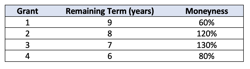
Table 1: Four Grants that Cliff Vest After Two Years

To use its historical data to derive an expected term for each of these grants, the historical data would need to contain options that were at similar levels. For example, ideally the company could study a collection of options that had 6 years left on their life and an in-the-money ratio of 80%. After all, this is exactly what’s underpinning a normal grant-date valuation insofar as you’re studying the homogenous pool of prior options granted and their behavior after being granted with a 10-year life and starting at-the-money.

In reality, very few companies can sub-segment their historical data to find representative prior grants that had comparable remaining lives and comparable moneyness levels at those same points in time.

So this is the problem: How do we come up with a supportable expected term assumption for a wide-ranging portfolio of grants, all of which have different remaining terms and different moneyness levels?

As we’ll note on multiple occasions, there can be a tension between how robust versus how simple of an approach to take. Robustness, where merited, yields greater precision and therefore reliability. More complex methods are not always better and, in the wrong contexts, can create an illusion of precision that reduces reliability. In such cases, simpler approaches can be more transparent and deliver a superior cost-benefit outcome. Navigating these tradeoffs is not new to financial accounting and ASC 718, specifically.

Let’s talk through a few approaches.

Midpoint Method

This is a variation on the SEC Simplified Method of ASC 718-10-S99-1, though we can’t call it the Simplified Method since that’s prohibited for options that don’t meet the plain-vanilla definition (including options not-at-the-money). Nonetheless, we can change the name and functionally adopt the same approach of calculating the midpoint between the weighted-average remaining time to vest and the expiration date. Basically, we split the difference between the earliest the option can be exercised and the latest it can be exercised.

Using our same options from above, let’s now add the resulting expected term:

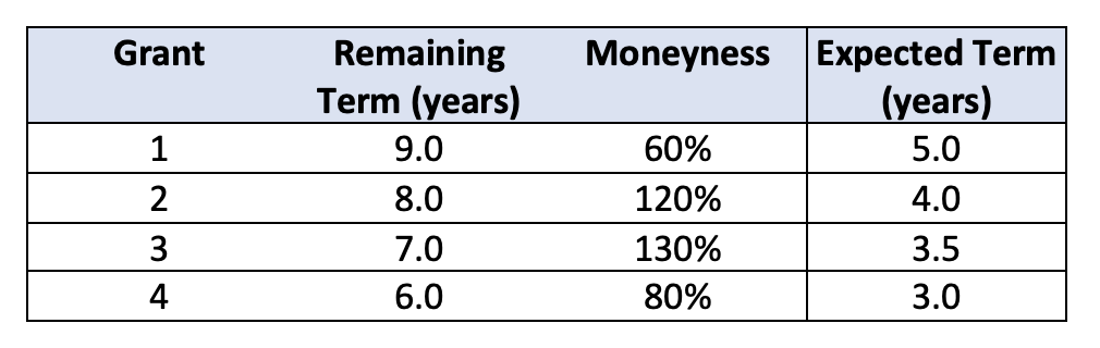
Table 2: Four Grants that Cliff Vest After Two Years under the Midpoint Method

You can probably see the problem. The math works fine, but how in the world would grant #4 get exercised earlier than grant #3? It’s got a lot more ground to cover to gain even a penny of value, whereas grant #3 is already in-the-money. As a spoiler alert, option exercise arguably has much more to do with moneyness than with raw time.

Let’s come back to the point about simplicity versus robustness. It may seem like this sort of an approach could never be appropriate. It depends. Even in a case like this involving a wide spectrum of moneyness levels, a more theoretically rigorous method could yield similar values based on the effect of other model assumptions or moving parts.

Contractual Term Method

Perhaps you’re bewildered by the underwater options and figure you’ll just use the remaining contractual term as a safe and conservative assumption. This is a second method that’s available.

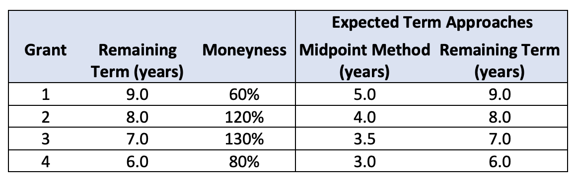
Table 3: Four Grants that Cliff Vest After Two Years under the Contractual Term Method

The problem is its reliability. For one, the remaining contractual term isn’t a realistic assumption for grants 2 and 3 which are already handsomely in-the-money. More concerning, this approach directly clashes with the paradigm being asserted on the date of grant. How can we say that a 10-year option that’s at-the-money will be exercised early, but a 7-year option that’s 30% in-the-money will be held until its expiration date?[3]

On page 64 of the final PvP rule, the SEC requires disclosure of the valuation assumptions used when those assumptions “materially differ from those disclosed at the time of grant.” Our concern with the contractual term method isn’t that we think it will trigger comment letters. Rather, the disclosure will be awkward because it will require dancing around the consistency problem noted above.

Elapsed Term Method

If the contractual term method concerns you because of its wobbliness on the underlying estimation paradigm, the elapsed term method can be a solution. Here we take the view that the expected term estimated at grant (which, in our example, is six years) remains reliable and is as good an estimate as any other alternative in light of the facts and circumstances. So we simply subtract the amount of time that has passed.

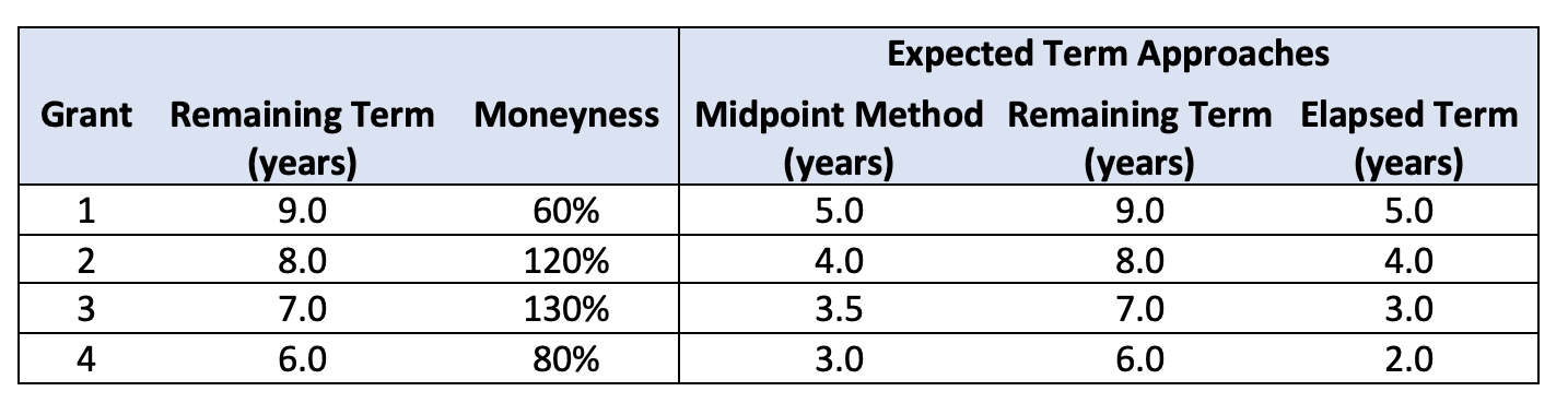
Table 4: Four Grants that Cliff Vest After Two Years under the Elapsed Term Method

But now we’re back to our original problem where we’re asserting that grant #4 is close to being exercised. It’s not. And grant #3 will certainly be exercised ahead of grant #4.

As we discuss throughout the paper, it’s important to explore whether such theoretical shortcomings matter in the context of the final results and whether more robust methods yield an uptick in reliability.

Elapsed Term Method with Adjustments

The elapsed term benefits from being simple, transparent, and consistent with the approach taken toward the grant-date fair value exercise. It may be the most appropriate model, but perhaps would benefit from adjustments that allow the expected terms to vary according to moneyness levels.

Various adjustments can be applied to the elapsed term method to fold in the effect of option moneyness. For example, the term could be linearly adjusted by the moneyness (stock/strike) ratio to shorten or lengthen the expected term based on the degree to which each option is in- or out-of-the-money. Alternatively, adjustments could be made to only deeply underwater options in order to maintain grant-date consistency for the bulk of the options while addressing the edge cases.

Such approaches have the benefit of directly taking moneyness into consideration, but they add another layer of subjectivity and complexity that may not make the results more accurate in a meaningful way. A thoughtful weighing of facts and circumstances is warranted when considering these alternatives, as always with valuations under ASC 718. Let’s jump to a different genre of tools: lattice models.

Lattice Model with Full Calibration

The customary way to implement a lattice model is to calibrate the full model on your historical data. If you have ample data, you’ll usually get a pretty robust result. If you don’t have much data, then you could calibrate the model using academic or other external data. In both cases, you still capture the primary benefit of adopting a model that produces expected term as an output.

**************

The Basics of Lattice Models

Lattice models are predicated on the same underlying financial economic theory as Black-Scholes. A lattice model built using an expected term assumption will give the same value as Black-Scholes (unless there are dividends, where Black-Scholes is commonly known to have a limiting flaw). Lattice models, however, are more flexible. They can be built with more inputs whereas Black-Scholes unconditionally has six inputs—no more, no less.

A simple lattice model uses a target in-the-money ratio to explain exercise behavior, such as asserting that employees will exercise once the stock price reaches 200% of the strike price. Far more elaborate lattice models can also be developed.

The elegance of a lattice model is that it can be run the same on options without adjustment regardless of remaining term or moneyness. In effect, it produces the expected term as an output instead of requiring it as an input. It models exercise behavior in the context of relevant parameters and outputs an expected term. In other words, it sidesteps the need to come up with an expected term as we try to do in the tables above.

**************

Assuming a 50% volatility, 0% dividend yield, and 4% interest rate, our table continues to expand.

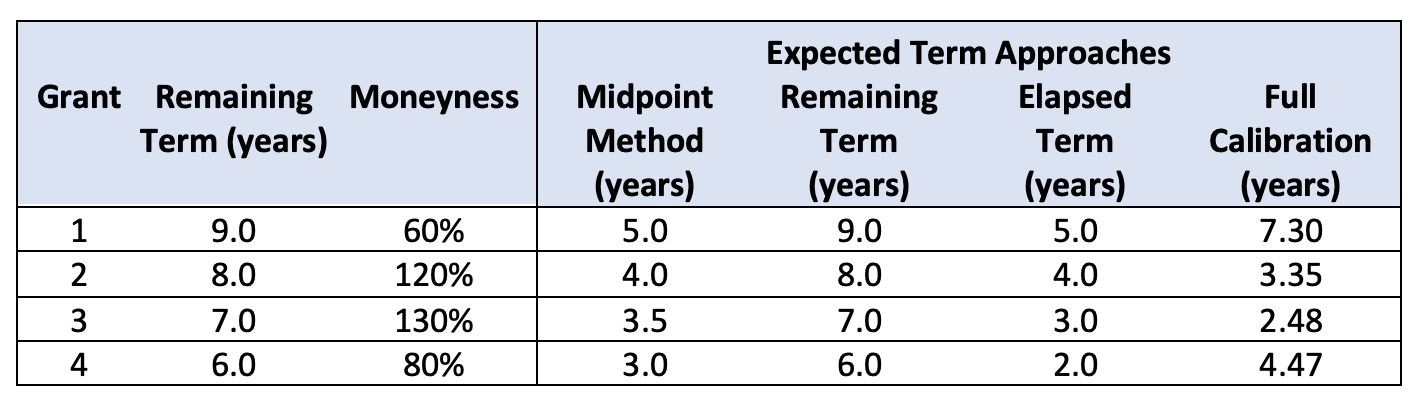
Table 5: Four Grants that Cliff Vest After Two Years under a Lattice Model with Full Calibration

The numbers look intuitive, but where did they come from? We used a simple Hull-White model where exercise is a function of reaching a particular in-the-money barrier, in this case 170% of the strike price. To get to a term, we then determined what term we could plug into a Black-Scholes in order to compare the model. Well, where did that come from? It came from an analysis of the company’s historical data.

Of course, we expect that companies using a lattice model for their grant date fair values will continue to do so for their PvP calculations.

All this is fine, and ASC 718 is explicitly clear in ASC 718-10-55-17 and 55-20 that it’s acceptable to use different models for different valuation circumstances. But this nonetheless requires added disclosure in the PvP footnotes since it represents a deviation in the assumptions from those used at grant.

Lattice Model with Calibration to Grant Date Fair Value

The last method involves a convenient technique offered in Footnote 55 of the original FAS 123R, now ASC 718-10-55-30. This method uses the Black-Scholes grant-date fair value to back-solve for the appropriate lattice model input (the in-the-money ratio). This way, the lattice model’s assumptions about exercise are directly, mechanically linked to those used in Black-Scholes at the point of grant. Importantly, we won’t see a value shift due solely to the model change. We’re simply using the lattice model to more objectively compute the expected term for later valuations in a way that’s consistent with the grant-date assumptions.

To do the math, we need one more input, the grant-date fair value in Black-Scholes. For simplicity, let’s assume that each of our two-year cliff vesting options was granted at $100 and had the same other inputs to yield a value of $52.42. This yields an in-the-money barrier of 2.27 and lets us fill out our final column in the table:

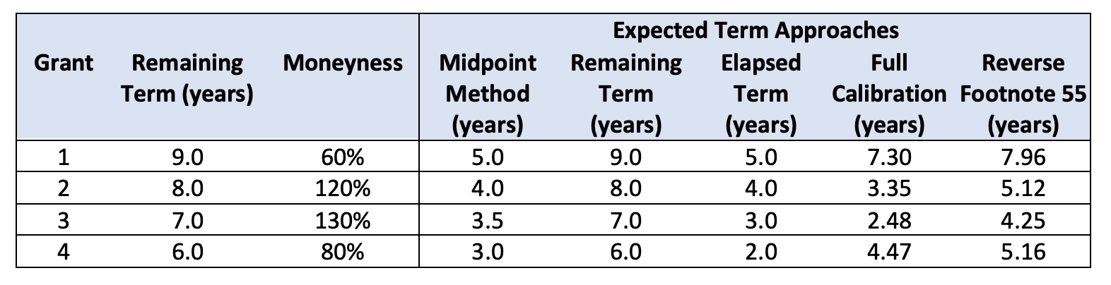
Table 6: Four Grants that Cliff Vest After Two Years under a Lattice Model with Calibration to Grant Date Fair Value

We used the same volatility and interest rate in every valuation, but as a practical matter, these would likely vary simply due to the passage of time. How would this method get disclosed? We envision language such as:

We used a binomial lattice model to value outstanding options included in the measurement of compensation actually paid. This allows us to estimate the value of each option in the context of each option’s remaining contractual life and in-the-money ratio at the point of measurement. To maintain consistency with our approach toward grant-date fair value estimation under ASC 718, we inferred the binomial lattice model’s exercise barrier from the Black-Scholes grant-date fair value. That input is an assumed in-the-money ratio at which exercise will occur, which is comparable to the model used throughout the illustrative examples in ASC 718.

Of course, there are other approaches to using a lattice model and estimating the expected term assumption. These include using data from academic research, actuarial research, and other tools for calibrating either a lattice model or Black-Scholes. But rather than building an excessively exhaustive list, let’s switch gears and cover how to compare and contrast the different approaches on the table.

How to Choose an Appropriate Technique

Our view is that you should begin with your fact pattern and bring all the available tools to the table. We’ve chosen not to vary our fees by approach, because technology lets us capture similar efficiencies and we think the decision should fit each company’s own context.

More often than not, the most effective methods turn out to be the Elapsed Term Black-Scholes and Reverse Footnote 55 Lattice. The Black-Scholes approach is crude but incredibly simple and transparent. The lattice approach is more complex but also much more precise and robust. We generally don’t prefer in-between approaches that add complexity for its own sake but still suffer from the same inherent flaws as the simplest models.

In all circumstances, it is key to weigh the valuation principles of ASC 718 to ensure that any valuations done for the pay vs. performance disclosure are compliant with US GAAP.

The SEC reiterated this at the 2022 AICPA and CIMA Conference on Current SEC and PCAOB Developments. Although not speaking on behalf of the SEC and not posted as a speech to the SEC’s website, Lindsay McCord noted that “Under Regulation S-K, we would expect that equity award fair value would be based on the principles of ASC 718” and that a registrant “could not rely on a method to determine the expected term assumption such as simply subtracting the elapsed actual life from the grant date expected term assumption without considering any of the other factors for determining expected term under US GAAP.”

This advice is consistent with our reading of the PvP rule, which suggests that a holistic analysis is needed of the relevant facts and circumstances. For some companies, a more robust model will be the right answer. For others, a simpler model may suffice perfectly well—it’s just critical to arrive at that answer via thoughtful consideration of relevant GAAP and not as a simplistic default.

Let’s look at two factors that can aid decision-making. First, do you pay a dividend yield and are your options in-the-money? If so, this may trigger one of Black-Scholes’ known flaws. Second, is there a wide spread of in-the-money levels? The more scattered they are, the more you’ll benefit from a more robust technique. We’ll cover these topics next.

Lattice vs. Black-Scholes: Dividends and Moneyness

A commonly understood problem with Black-Scholes is the manner in which it treats dividends. This problem is accentuated when an option is in-the-money.

Let’s start with an example considering an option at its vesting date:

• Current stock price: $40
• Strike price: $20
• Expected term (years): 6

• Volatility: 30%
• Risk-free interest rate: 3%
• Dividend yield: 4%

This option’s intrinsic value is $20. Using these assumptions, Black-Scholes produces a fair value of $16.50 because it assumes the option will be held to maturity, and the option holder loses the value of six coming years of dividends. Indeed, the holder could exercise the option today and get $20, which sets a floor for the value and means that Black-Scholes would not be ASC 718-compliant in this case.[4]

The second factor that can influence the model selection decision is the presence of a wide spectrum of strike prices, and specifically underwater options. The logic is that an option’s moneyness influences exercise decision-making, and therefore in certain fact patterns the valuation technique should somehow incorporate moneyness in its determination of exercise behavior. A lattice model does this most elegantly, but as noted, certain adjustment could be applied to a basic Black-Scholes approach.

These issues are most salient in the context of a critical mass of deep underwater options. While the theory may suggest moneyness always influences exercise behavior, these cause-and-effect relationships are more nebulous in the context of in-the-money options. Executives holding a wide spectrum of in-the-money options face a complex array of decisions, including share ownership targets, tax planning, broader goals to hold closer to term, lumpy liquidity needs, etc. Additionally, deep-in-the-money options derive most of their value from the intrinsic value and not the time value.

Deep underwater options are much different, especially as you think about the likely exercise behavior in relation to the original grant date expected term. Suppose an option is 90% underwater, the original expected term was six years, and the option is two years into its life. In this case, it’s genuinely less realistic that the option will be exercised in four years—it may not even be at-the-money in four years. Therefore, either an adjustment for moneyness or a lattice model that explicitly models exercise behavior in the context of moneyness could be appropriate.

But even here we need to be measured and not imbue an illusion of precision. Suppose an option is only 30% underwater. Remember that the original grant date expected term is a weighted-average best-guess of how long an option is likely to be alive. These calculations factor in post-vesting cancellations where an option expires underwater after its ten years. Additionally, even if an option is 30% underwater, with a high volatility, circumstances can quickly change. We also know that risk aversion influences exercise behavior, and an option that recovers from being underwater is most likely to trigger risk averse tendencies to exercise early.

None of these are causal statements, but rather, a cautionary note about imbuing too many complex assumptions and adjustments when the fog of war is quite high.

For these reasons, the valuation professional needs to weigh the benefits of incremental precision, the subjectivity of any such on-top adjustments, the implications of using a different model for PvP valuation (e.g., lattice) than the model used for regular ASC 718 valuation (e.g., Black-Scholes), and other relevant principles in ASC 718.

This is why we encourage you to be leery of simplistic, one-size-fits all approaches, and devote the time to considering multiple approaches so that you can balance the tradeoffs and arrive at a methodology that best fits your fact pattern.

ASC 718 and PvP Valuation Model Differences

The question often arises as to whether a different valuation technique can be used for PvP than that used for ordinary course ASC 7178 grant date valuations. We believe the answer is “yes” given ASC 718-10-55-17 (and other similar references):

“The selection of an appropriate valuation technique or model will depend on the substantive characteristics of the instrument being valued.  Because an entity may grant different types of instruments, each with its own unique set of substantive characteristics, an entity may use a different valuation technique for each different type of instrument.”

Options with markedly different moneyness levels could be construed as having different substantive characteristics, thus meriting the use of a different model. The PvP rule requires disclosure and footnoting of any assumptions used that differ from those used at the grant date. All else equal, then, we think there is a benefit to maximizing consistency to the grant date fair value method when doing so doesn’t result in a material downgrade to reliability. Consistency will be clearer and more intuitive to a user of the PvP table who would most likely expect there to be symmetry in approach.

Along these same lines, consider whether you have had historical award modifications, assumed options in a business combination, or option grants that are underwater and therefore have a de facto market condition. We suggest thinking of the PvP valuation as part of a broader strategy on how to treat unique situations that involve fact patterns that diverge from those present in ordinary course ASC 718 valuations.

Lattice vs. Black-Scholes: Year-over-Year Swings

The impact of model selection on valuation is fairly straightforward:

• If the stock price goes up, we expect the value of the option to go up, and conversely for a falling stock price
• Further, options are leveraged instruments, meaning that if the stock price goes up (say by 10%), we expect the option value to move by more than this
• On the other hand, as time passes, the option value goes down. The remaining chance for the stock price to move up (or alternatively, the insurance value of being able to walk away in a down market) reduces. In option parlance, this is called theta bleed, theta being the term for the movement in option value over time[5]

As discussed above, one would intuitively expect an increasing price to result in a shorter holding period. As a result, this shorter term mitigates the change in value from the stock price alone. Lattice models allow us to capture this effect and reflect smaller year-over-year value variance.

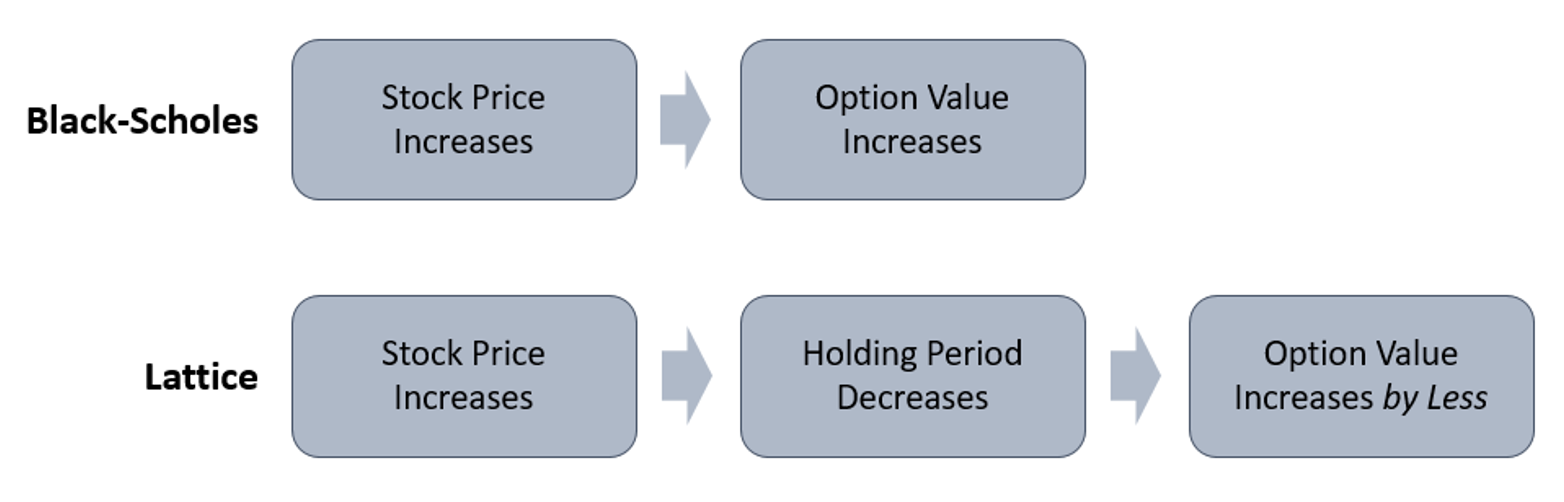
Figure 1: Lattice vs. Black-Scholes Models

For a stock price decrease, the impact is reversed. In order to show the impact, we show the results comparing two models.[6]

• The first is a Black-Scholes model using the elapsed term method. This assumed a seven-year expected term at the grant date, and at the end of a year, it assumes six years remaining.
• The second is a lattice model which assumes exercise at the end of the period, or if the stock price rises to 150% of the strike. Because higher stock prices are closer to the hurdle, this will shorten the term in these cases.

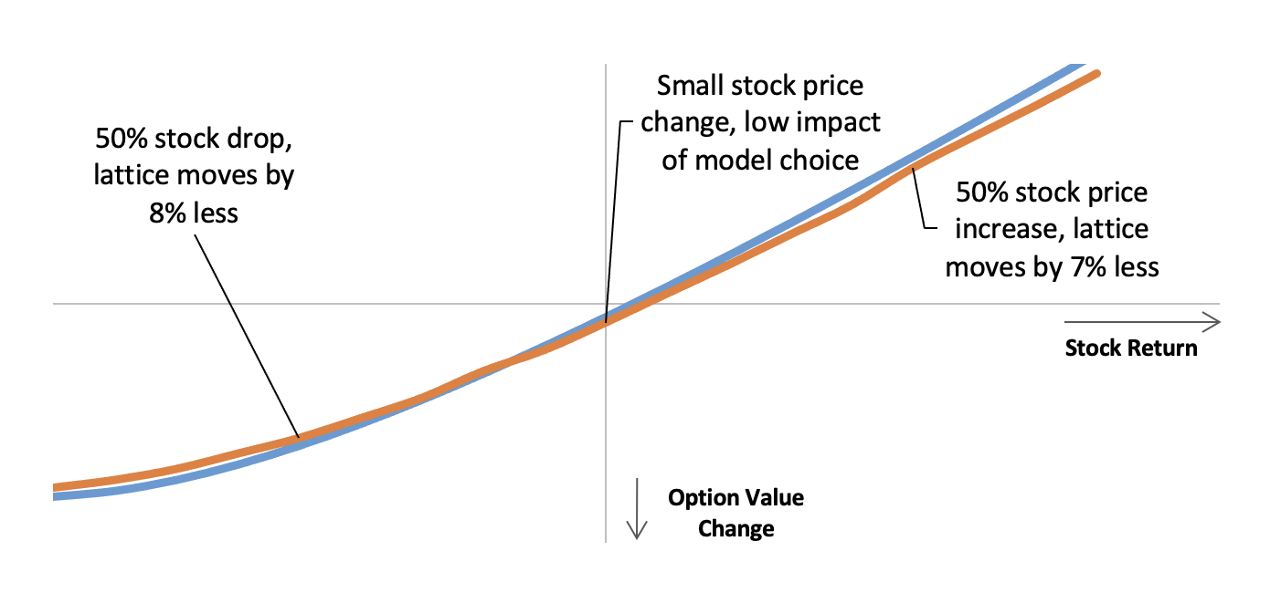
Figure 2: Option Value Moves under Lattice vs. Black-Scholes Models

The results show exactly what we anticipated. If the stock price stays flat, we see a low drag on the option value from the passage of time, approximately 3%. The stock needs to go up around 5% to keep the value neutral.

On both sides of the curve, we see the lattice value results in a smaller impact than the Black-Scholes value. In our example, we see this is frequently in the 7-8% range, meaning this could show a definite impact on the disclosed figures, especially for companies with a large portion of their compensation as options.

Of course, your mileage may vary. But the point is that in some contexts lattice models may give a strategically more desirable result (while also being more accurate). The cons could outweigh that benefit, which is why it’s good to consider the full spectrum of alternatives.

Final Thoughts

Equity award valuation is proving to be the most complex piece in the calculation of CAP. TSR awards require separate Monte Carlo models that are built to capture the distinct terms of each award. Options are different because they’re all the same (e.g., 10-year term) and are simply at different points in their life and at different moneyness levels, referred to as being “on the run.”[7]

Given this homogeneity in option terms, the best valuation method is the one that can mass-process the entire portfolio of options subject to the PvP calculation, yield reliable results for each option, and require minimal to no hunting and pecking through individual results because they’re contradictory or unreliable. The model that accomplishes that could be Black-Scholes. On the other hand, Black-Scholes could also be the source of unsupportable results, such as some of the cases we reviewed in this paper.

That’s why our approach with clients is to look at the data first, then evaluate the right tradeoff between model rigor and model simplicity. We make it our clients’ decision, we offer our recommendation and perspective, and we intentionally don’t vary our fees by the decision. The goal is for you to develop a methodology that’s efficient, scalable to all your options subject to the CAP calculation, and supportable, with a clean disclosure.

If you have any questions about this new rule and how it impacts your company, feel free to reach out.

[1] Typical reasons for early exercise include liquidity needs, risk aversion and the inability to hedge risk as holders of tradable options can do, and departure from the company.

[2] The moneyness level is the ratio of the current stock price to the strike price. For example, a moneyness of 70% means that if the current stock price is $7, the strike price is $10.

[3] Some companies use a contractual term for their options at grant for NEOs and other senior employees. For these, we believe that maintaining this makes the most sense.

[4] The Cox, Ross, Rubenstein lattice model takes into account optimal exercise incorporating future dividends, and can be implemented into the aforementioned lattice with a stock price hurdle to capture optimal as well as employee “sub-optimal” early exercise.

[5] We note that theta bleed would also be a great name for a punk rock band and/or action movie franchise.

[6] We assume the option is at the money, stock and strike is at $0 at the grant date, and the term is a full year. Our option cliff vests in 4 years and expires in 10. Volatility is 35%. Risk-free rate is 2%. Our stock does not pay dividends. Post-vest termination rate in our lattice model is 2%.

[7] While we’re not aware of a band named after Theta Bleed, it’s conceivable that REO Speedwagon and/or Paul McCartney and Wings had some exposure to valuing options on the run.