Real World vs. Risk Neutral: Understanding the Difference between Valuation and Derived Service Period Assumptions

As we frequently deal in unique valuation problems, the question “What world are you living in?” is sometimes hurled at us, we hope in jest. However, seemingly silly questions often uncover a bigger truth. In this case—the world of derivative valuation—we truly aren’t living in the real world. In fact, our valuations are based on a hypothetical world where all investors are “risk neutral.” While this works for valuation, it causes some confusion when considering the derived service period, which is based on the time to vest. To understand why, let’s first review how risk-neutral valuation works for derivatives.

Risk-Neutral Valuation

The sharp-eyed reader of ASC 718 will notice ASC 718-10-55-11, which (seemingly innocuously) states:

If observable market prices of identical or similar equity or liability instruments of the entity are not available, the fair value of equity and liability instruments awarded to employees shall be estimated by using a valuation technique that meets all of the following criteria:

b. It is based on established principles of financial economic theory and generally applied in that field (see paragraph 718-10-55-16). Established principles of financial economic theory represent fundamental propositions that form the basis of modern corporate finance (for example, the time value of money and risk-neutral valuation).

This guidance seemingly glosses over two concepts:

1. The time value of money. Everyone pretty much understands that money today is worth more than money tomorrow (with the notable exception of some recent negative interest rate environments in Europe).

2. Risk-neutral valuation. Risk-neutral valuation says that when valuing derivatives like stock options, you can simplify by assuming that all assets grow—and can be discounted—at the risk-free rate. In fact, this is a key component that can be used for valuation, as Black, Scholes, and Merton proved in their Nobel Prize-winning formula.

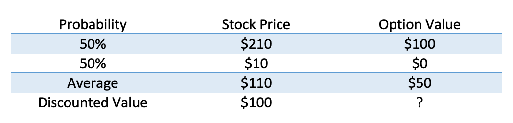
What do these concepts, put together, really mean? Let’s take a stock, Coin Flip Enterprises (ticker: FLIP). FLIP is trading at $100 today, and the expectation is that in one year they will trade at either $10 or $210 with equal probability.[1] Straightforward math shows the average future price is $110 and the expected return is 10%, a reasonable return for a share of stock.

Now let’s think of a one-year stock option on FLIP granted with a strike of $110. At expiration, the option value can be $100 or $0, and the average value is $50. But our question is: What is that option worth today? If we discount it based on the same 10% growth rate, we get to $45.45, but the option is no doubt riskier than the stock as it leaves the opportunity to get left with nothing. Therefore, investors would demand a higher return.

We can get the same result if we combine stocks and borrowing into a so-called replicating payoff with the same payout. For example, imagine I buy a half of a share of FLIP stock and borrow an amount such that I owe $5 in the future.

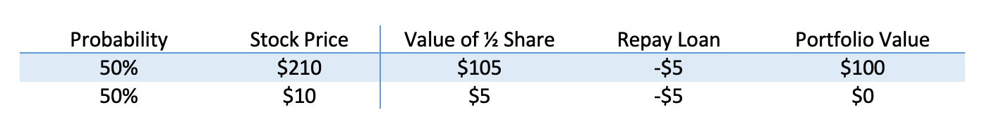
Note that it costs $50.00 to buy half a share of stock, but I borrowed $5, assuming no interest. That means that for $45.00, we can have this exact same payoff, so that must be the value of the option. The expected return for this is 11%, but we would have had no way to know that if we hadn’t done this math.

But say I make a quick adjustment. Instead of having the stock grow at 10%, we grow it at our (non-existent) risk-free rate.

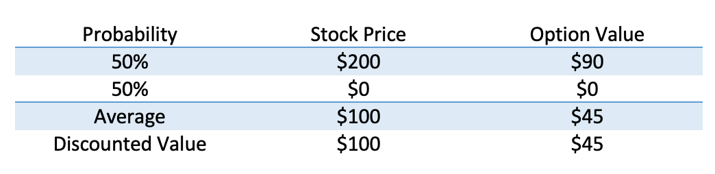
The value, $45 is the same as the cost of the replicating portfolio.

There are a few interesting facts here:

• The probability never really mattered. In fact, the stock’s expected rate of return didn’t matter at all, just the stock price.

• You can do this for any option strike price. If the outcomes and the risk-free rate are the same today, the stock price doesn’t matter either.

• If there are more steps, we can keep rebalancing our portfolio. (This is the core of a lattice model, while Black-Scholes-Merton assumes this rebalancing happens at infinite frequency.)

From here on, the math gets complicated, but the takeaway is the same. Because we can use these replicating portfolios, we can work around risky rates of return in our valuation models, instead reducing everything to the risk-free rate.

Shifting to the Real World

Risk-neutral valuation works well for valuing derivatives. It does not, however, work well for accurately forecasting the time to hit a stock price target because assets are modeled to grow at an artificially low rate. As the adage goes: higher risk, higher reward. Stocks must grow on average at a higher rate than a risk-free asset, which means that in a risk-neutral world, it takes stock longer to hit price targets. Therefore the valuation model used for price hurdles and similar awards results in prices that are lower than an investor would actually expect to see.

It’s important to note that this can have an impact on a more accurate calculation of the derived service period. Recall that the derived service period is the median path among those that vest. Because this is based on the expected time to vest, it can make sense to use a real-world service period. This requires a second Monte Carlo simulation, identical to that used for valuation except with a higher growth rate.

Shifting to the real world in looking at time has two effects. The first is on the Monte Carlo simulation paths that vest. Given a higher growth rate, they vest earlier using a higher real-world cost of equity (see Figure 1 for a sample average path in both environments).

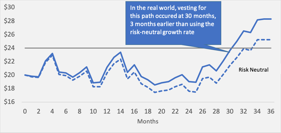
Figure 1: Share vests earlier in a real-world trial

The second effect is that the stock price increases more so that more paths vest in the real world than we forecast, given the higher returns (see Figure 2).

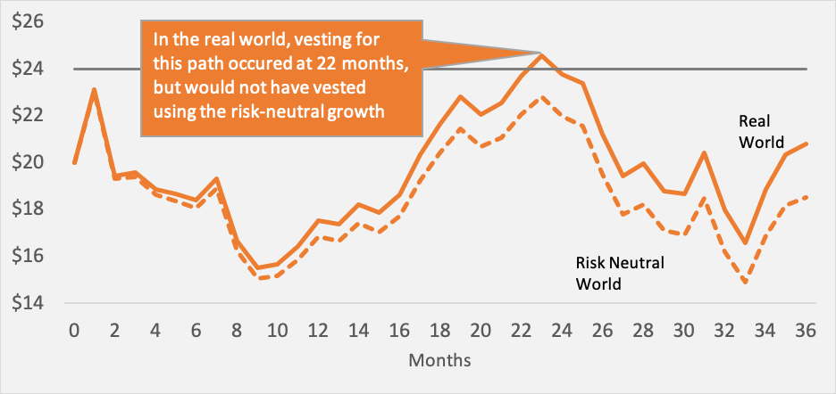
Figure 2: More paths vest in a real-world trial

Now, you may recall that the derived service period is the median term for those paths that vest. So if more paths vest, but paths take less time, the derived service period could go either way. In fact, we usually see the term go down as the first factor has a larger impact. As a result, using a real-world cost of equity for the estimation of a derived service period results in a shorter expense recognition term and an effective acceleration of the expense.

Valuations Based on Real-World Inputs

Occasionally a valuation will depend on a real-world metric. For example, in the valuation of contingent considerations following a transaction, it’s not uncommon to see a payout based on the future revenue or EBITDA of the target company. In these cases, it’s no longer possible to use the replicating portfolio logic or the analog that all asset prices grow at the risk-free rate. The reason is that EBITDA is not an asset, and companies’ expectations are not developed in the risk-neutral world.

In these cases, an adjustment is used to bridge between the real world and our risk neutral framework. This typically entails discounting future cash flows to reflect the riskiness of these, so that a risk-neutral equivalent can be used.

The upshot? All types of valuation require models and assumptions. A familiarity with both can help to avoid skewing the results or presenting information which is too easy to misinterpret.

[1] Of course, these numbers are selected to make the math easier to see. When an option valuation is performed, it’s typically assumed that the underlying stock return follows a normal distribution. The expected future stock prices are based on this assumption and the expected volatility of the stock. In essence, it’s like an infinitely large numbers of coin flips.